
The Search for Renewables in Tech and Beyond.
9 OctBuying Renewable Power for Data Centers Poses Major Challenges for Internet Companies
 Google
In some cases, it’s legal roadblocks. In other cases, it’s the internet companies themselves.
Bentham Paulos
October 8, 2014
The internet lives inside a nondescript big-box building on the outskirts of Council Bluffs, Iowa. Only a set of primary-colored stripes gives a clue that it houses a Google data center.
The building is full of computers, mounted on racks in row after row, busy serving up cat videos, web searches, email and countless other digital packets.
The building uses massive amounts of electricity — enough to power a city of 30,000 homes. Power use is so critical to data centers that their size is measured by watts of electricity, not by megabytes or square feet.
When Google started to develop the data center, Iowa was largely coal-powered, making the data center’s carbon footprint much bigger than the company wanted it to be. Google calculated the regional carbon intensity at 0.739 kilograms of CO2 per kilowatt-hour, making its annual footprint about 260,000 metric tons of CO2 — far out of line with the company’s corporate sustainability goals.
An increasing number of IT companies are finding themselves in the same situation.
Cloud computing, where applications and files are stored on remote servers instead of on your local computer, is getting bigger. Greenpeace calculates that the cloud used an estimated 684 billion kilowatt-hours in 2011, enough to rank it sixth among countries. That number will increase 63 percent by 2020. Internet data growth is expected to triple between 2012 and 2017, driven by a 50 percent increase in users and increasing traffic for streaming video and audio.
At the same time, many IT companies have big sustainability goals. They are seeking to increase energy efficiency at their data centers, increase transparency in public communications and buy more renewable energy. Apple, Box, Facebook, Google, Rackspace and Salesforce have all committed to 100-percent-renewable-energy goals.
“Focusing on energy is a relatively easy thing for companies to do to increase sustainability,” said Gary Cook, an IT analyst for Greenpeace. “Renewable energy is increasingly affordable, sometimes even cheaper than conventional power. It’s much more difficult to influence their supply chain, like Wal-Mart has been doing.”
Google took extraordinary measures to make it work, getting licensed as a power wholesaler so it could directly buy power from Midwest wind farms. For its Council Bluffs center, the company buys power from a NextEra wind farm near Ames, Iowa.
Google then sells the power back to the local utility and retires the renewable energy certificates (RECs). “This may result in a slight net loss for Google,” the company points out, “but we expect the contract to eventually make money as power becomes more expensive over time.”
To make everything transparent and provide leadership in the IT world, Google wrote up the idea and process in a white paper it posted online.
Google now has a team of 30 working on renewable energy procurement and investment, but few other companies have the ability to go to such lengths.
The IT companies, as well as many other corporations with sustainability goals like Walmart, Walgreens and REI, have encountered a tangle of challenges in buying renewable power, especially in states with regulated utilities. The easiest workaround has been to buy RECs that have been separated or “unbundled” from the underlying power.
But RECs are falling out of favor, since they lack two critical features that many buyers want. First, they may come from power plants that might have been built anyway; in the jargon of carbon-tracking, they lack “additionality.”
Second, the customer still buys local “brown” power, and the RECs are an expense on top of that. They don’t give the customer the fixed-price guarantee that a wind or solar generator can deliver.
As a result, companies are looking for new ways to buy renewables. In addition to Google’s wholesale PPA approach, buyers are using special green tariffs, signing “contracts for differences” to get a financial hedge and also doing onsite generation. A number of the companies are working with World Resources Institute, World Wildlife Fund and Business for Social Responsibility (BSR) to explore new approaches.
To help with the process, Rocky Mountain Institute is getting ready to launch a Business Renewables Resource Center. The center will act like a travel agent, guiding corporate buyers through the arduous process of buying renewables.
One novel approach may be available soon. To make it possible to both meet corporate climate goals and site a new data center in Utah — which has a power system dominated by coal — eBay helped push legislation there that allows direct sales of renewables in a state that is otherwise fully regulated.
The Utah Public Service Commission is now going through a rulemaking process and encountering resistance from regulators and Rocky Mountain Power worried about cost shifting. “Rocky Mountain Power’s tariff proposal is completely unworkable,” said Sarah Wright, director of Utah Clean Energy.
The legislation opens the door to other customers beyond the IT sector. Powdr Corp., which owns eight ski resorts, and Wal-Mart, with 54 stores in Utah, are both intervening in the docket.
Brent Giles of Powdr Corp. wrote in a filing about the proposed legislation, “[We] hoped SB12 would help us to develop a fair and simple method to enable us to continue to make investments for more clean energy in Utah.”
But proponents of the direct sales law say a raft of proposed fees from Rocky Mountain Power are intended to thwart the process. Wal-Mart calculated that it “would spend $291,600 a year just for costs from the administrative fee,” not to mention the various other fees.
However, David Eskelsen, a spokesman for Rocky Mountain Power defended the proposed fees, saying that commission staff “reviewed and verified the company’s calculations for the billing and metering charges, and for the delivery and backup service charges.”
Cheryl Murray, an analyst at the Utah Office of Consumer Services, wrote in a filing that cost shifting was a potential problem: “The Office is concerned that some parties may be seeking lower costs rather than more accurate costs. While we understand this desire, lower costs for Schedule 32 customers must not come at the expense of other customers.”
On the contrary, Iowa rolled out the red carpet to attract Facebook. MidAmerican Energy worked with Facebook to ensure that the company’s new Iowa data center, now under development, would be entirely powered by local wind. The project is part of the biggest purchase of wind turbines in history — a $1.9 billion, 1,050-megawatt order was placed last year with Siemens.
Apple and Microsoft have also executed big renewables deals. Apple’s North Carolina operations are powered by a mix of ground-mounted solar — 40 megawatts currently, set to increase to about 60 megawatts — and fuel cells that run on biogas. It has also announced that iPhone 6 screens are being made in a solar-powered factory.
Microsoft says it hit the 100-percent-renewable mark last year, buying power from wind farms in Texas and Illinois, hydro plants in Washington and biogas in Wyoming (though much of the total comes from buying RECs). It has also worked with the University of California, Irvine to integrate fuel cells into a data center, mounted on racks alongside the servers. “We were able to boost the electrical efficiency of our fuel cell system from 39.8 percent to 53.3 percent by cutting out much of the electrical conditioning systems,”Microsoft reported in February.
Notably missing so far are Amazon and Twitter, as well as “server hotel” companies like Equinix and Digital Realty. Amazon Web Services is the largest data center company, delivering for dozens of clients, including Yelp, Vimeo, Spotify and Netflix. By one measure, Netflix accounts for 34 percent of web traffic during peak times in North America.
Amazon recently hired its first director of sustainability. The efforts it will undertake in the sustainability space remain unknown, however, since Amazon is famously tight-lipped about corporate operations and plans. Twitter, meanwhile, received an “F” from Greenpeace for its sustainability goals, achievements and disclosure practices.

Wearable Technology…. YES!!!
30 Mayhttp://www.youtube.com/watch?v=UeP0qeiwHjk
From MEMS technology to the nuances of “Things to Wear”. We are finding more ways to stay connected. The notion of the funnel of “Big Brother” is now beginning to be inverted to “Big Individual”. Small personal devices link to Clouds and virtual life tools, specifically tailored to the individual. Big Brother has No Clothes and No teeth. But who is really paying close attention to this transformation. Well, I am. I hope you are as well. Let me know what you think about the death of the Big Brother syndrome.
This is the start of the Internet of Things (IoT) and leading to the Internet of Everything (IoE). Energy independence and fair costs based upon the new energy economy. SD1 Incorporated and it’s new LEXI™ Bundled services platform is the forerunner of things to come.
Stay Tuned.
Internet of Things (IoT), INTEL and INTEL stakeholders and developers. Internet of Everything (IoE) Cisco and Cisco stakeholders developers.
1 A
28 Mar
We need to seek to be 1 A in our effort to solve the challenges inherent with Climate Change.
Here is a recent graphic generated by Michelle St.P (Ross) for SD1 Incorporated. The 1 A position in service is a take off from the selective service classification of the United States. [http://en.wikipedia.org/wiki/Selective_Service_System] However, the 1 A listing can apply to being available for service in the effort to face the 21st Century challenges of Climate Change and new energy technology for our human family. Climate Change can not be ignored. We must work together on solutions not disputes.
http://sd1.co, http://facebook.com/sd1, Project – SD1 R&D
A Key Innovation
26 MarA Key to innovation is the creative process. This overview shows interesting overlaps and disruptive elements of group innovation.
http://www.petertenhoopen.com/rs_creativity.phpHow to create creative organizations
Peter ten Hoopen employs a four step approach:
- Diagnostics – Chart the Organisation’s Creativity
We plot the organisation’s Creativity Index using our Creative Culture Survey (CCS), a fine-grained look at the factors promoting and inhibiting creativity and innovation in the team, department or entire organisation. Low cost, very effective in opening up discussion and forcing reflection.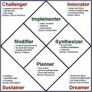 Either in parallel or separately we use our Innovation Roles Model (IRM), which identifies eight different roles people play in a field outlined by the axes of Creativity and Risk-Readiness. Builds on work by Belbin, Byrd and Lockwood Brown. All our work on innovation is linked to leadership.
 - Validation – Analyse and Discuss the Outcome
To be accepted, results need to be analysed and validated (and where necessary fine-tuned) in workshops – highly interactive. Is this really who we are? Are we happy with it? If not, how do we change? - Change – Breakthrough Initiatives
Appoint change teams to come up with initiatives that provide real breakthroughs in terms of the organisation’s or the group’s attitude towards creativity. What do we need to do to open up our minds? How do we best apply our energy? And who is ready to take ownership for agreed changes? Who shows real leadership? Uses Innovation Roles Model to create strong teams of people who understand one another’s role, and become mutually supportive. - Root – ‘Keep the Change’
Our idea is to help organisations help themselves. We just provide the framework, the tools, the spark, the facilitation. Once that is done, we get out of your way. The change is yours to keep. And to maintain. Lasting change is achieved through our Values to Performance Program – highly engaging workshops in which participants jointly agree to commit themselves to behaviours that they themselves support. Creates awarenes of creative potential, awareness of one’s own limiting factors and a sense that these can be overcome, particularly by working with others. Also sets out guidelines that prevent backsliding into non-productive, creativity limiting behavior.
A* Prime
3 Sep
Heads Up. We write along to right a wrong and to be a peace-maker.
From: BlindFiveYearOld.
http://www.blindfiveyearold.com/how-to-implement-rel-author
Overshadowed by the Google+ launch was the implementation of the rel=author markup in search results. Once implemented, authors are given a very prominent treatment on search results.
Three Link Monte
The TL;DR version for implementing rel=”author” is that it requires three specific links.
- A link from your blog post or article to your author page using rel=”author”
- A link from your author page to your Google profile page using rel=”me”
- A link from your Google profile page to your author page using rel=”me”
Read on for specific directions on how to get rel=”author” up and running on your own site or blog.
THE MICROGRID PRIMER EVERY POWER ENGINEER SHOULD STUDY, ANALYSIS, ANALYTICS, AND INTEROPERABILITY RULES. THESE GUIDING PRINCIPLES CAN HELP MINIMIZE FRICTION: · DEFINE…
View original post 566 more words
A* String support for Key for Web Developers
29 Aug
A* String Support
A* String
http://en.wiktionary.org/wiki/A*_String
https://plus.google.com/b/117046733826562293702/dashboard/overview
NACIS
541711 Research and Development in Biotechnology
This U.S. industry comprises establishments primarily engaged in conducting biotechnology research and experimental development. Biotechnology research and experimental development involves the study of the use of microorganisms and cellular and biomolecular processes to develop or alter living or non-living materials. This research and development in biotechnology may result in development of new biotechnology processes or in prototypes of new or genetically-altered products that may be reproduced, utilized, or implemented by various industries.
Check out the resource(s) at A List Apart. Key tools for web development and website development.
___________________________
Wikipedia, Justin Bieber,
https://plus.google.com/110458508713292000394/posts/PqFJvBwNC81
http://en.wikipedia.org/wiki/A*_search_algorithm
| Graph and tree search algorithms |
|---|
| Listings |
| Related topics |
In computer science, A* (pronounced “A star” ( listen)) is a computer algorithm that is widely used in pathfinding and graph traversal, the process of plotting an efficiently traversable path between points, called nodes. Noted for its performance and accuracy, it enjoys widespread use. (However, in practical travel-routing systems, it is generally outperformed by algorithms which can pre-process the graph to attain better performance.[1])
Peter Hart, Nils Nilsson and Bertram Raphael of Stanford Research Institute (now SRI International) first described the algorithm in 1968.[2] It is an extension of Edsger Dijkstra’s1959 algorithm. A* achieves better time performance by using heuristics.
and more on pathfinders – http://www.policyalmanac.org/games/aStarTutorial.htm
A* Pathfinding for Beginners
By Patrick Lester (Updated July 18, 2005)
This article has been translated into Albanian, Chinese, French, German, Portuguese, Romanian, Russian, Serbian, and Spanish. Other translations are welcome. See email address at the bottom of this article.
The A* (pronounced A-star) algorithm can be complicated for beginners. While there are many articles on the web that explain A*, most are written for people who understand the basics already. This article is for the true beginner.
This article does not try to be the definitive work on the subject. Instead it describes the fundamentals and prepares you to go out and read all of those other materials and understand what they are talking about. Links to some of the best are provided at the end of this article, under Further Reading.
Finally, this article is not program-specific. You should be able to adapt what’s here to any computer language. As you might expect, however, I have included a link to a sample program at the end of this article. The sample package contains two versions: one in C++ and one in Blitz Basic. It also contains executables if you just want to see A* in action.
But we are getting ahead of ourselves. Let’s start at the beginning …
Introduction: The Search Area
Let’s assume that we have someone who wants to get from point A to point B. Let’s assume that a wall separates the two points. This is illustrated below, with green being the starting point A, and red being the ending point B, and the blue filled squares being the wall in between.
[Figure 1]
The first thing you should notice is that we have divided our search area into a square grid. Simplifying the search area, as we have done here, is the first step in pathfinding. This particular method reduces our search area to a simple two dimensional array. Each item in the array represents one of the squares on the grid, and its status is recorded as walkable or unwalkable. The path is found by figuring out which squares we should take to get from A to B. Once the path is found, our person moves from the center of one square to the center of the next until the target is reached.
These center points are called “nodes”. When you read about pathfinding elsewhere, you will often see people discussing nodes. Why not just call them squares? Because it is possible to divide up your pathfinding area into something other than squares. They could be rectangles, hexagons, triangles, or any shape, really. And the nodes could be placed anywhere within the shapes – in the center or along the edges, or anywhere else. We are using this system, however, because it is the simplest.
Starting the Search
Once we have simplified our search area into a manageable number of nodes, as we have done with the grid layout above, the next step is to conduct a search to find the shortest path. We do this by starting at point A, checking the adjacent squares, and generally searching outward until we find our target.
We begin the search by doing the following:
- Begin at the starting point A and add it to an “open list” of squares to be considered. The open list is kind of like a shopping list. Right now there is just one item on the list, but we will have more later. It contains squares that might fall along the path you want to take, but maybe not. Basically, this is a list of squares that need to be checked out.
- Look at all the reachable or walkable squares adjacent to the starting point, ignoring squares with walls, water, or other illegal terrain. Add them to the open list, too. For each of these squares, save point A as its “parent square”. This parent square stuff is important when we want to trace our path. It will be explained more later.
- Drop the starting square A from your open list, and add it to a “closed list” of squares that you don’t need to look at again for now.
At this point, you should have something like the following illustration. In this illustration, the dark green square in the center is your starting square. It is outlined in light blue to indicate that the square has been added to the closed list. All of the adjacent squares are now on the open list of squares to be checked, and they are outlined in light green. Each has a gray pointer that points back to its parent, which is the starting square.
[Figure 2]
Next, we choose one of the adjacent squares on the open list and more or less repeat the earlier process, as described below. But which square do we choose? The one with the lowest F cost.
Path Scoring
The key to determining which squares to use when figuring out the path is the following equation:
F = G + H
where
- G = the movement cost to move from the starting point A to a given square on the grid, following the path generated to get there.
- H = the estimated movement cost to move from that given square on the grid to the final destination, point B. This is often referred to as the heuristic, which can be a bit confusing. The reason why it is called that is because it is a guess. We really don’t know the actual distance until we find the path, because all sorts of things can be in the way (walls, water, etc.). You are given one way to calculate H in this tutorial, but there are many others that you can find in other articles on the web.
Our path is generated by repeatedly going through our open list and choosing the square with the lowest F score. This process will be described in more detail a bit further in the article. First let’s look more closely at how we calculate the equation.
As described above, G is the movement cost to move from the starting point to the given square using the path generated to get there. In this example, we will assign a cost of 10 to each horizontal or vertical square moved, and a cost of 14 for a diagonal move. We use these numbers because the actual distance to move diagonally is the square root of 2 (don’t be scared), or roughly 1.414 times the cost of moving horizontally or vertically. We use 10 and 14 for simplicity’s sake. The ratio is about right, and we avoid having to calculate square roots and we avoid decimals. This isn’t just because we are dumb and don’t like math. Using whole numbers like these is a lot faster for the computer, too. As you will soon find out, pathfinding can be very slow if you don’t use short cuts like these.
Since we are calculating the G cost along a specific path to a given square, the way to figure out the G cost of that square is to take the G cost of its parent, and then add 10 or 14 depending on whether it is diagonal or orthogonal (non-diagonal) from that parent square. The need for this method will become apparent a little further on in this example, as we get more than one square away from the starting square.
H can be estimated in a variety of ways. The method we use here is called the Manhattan method, where you calculate the total number of squares moved horizontally and vertically to reach the target square from the current square, ignoring diagonal movement, and ignoring any obstacles that may be in the way. We then multiply the total by 10, our cost for moving one square horizontally or vertically. This is (probably) called the Manhattan method because it is like calculating the number of city blocks from one place to another, where you can’t cut across the block diagonally.
Reading this description, you might guess that the heuristic is merely a rough estimate of the remaining distance between the current square and the target “as the crow flies.” This isn’t the case. We are actually trying to estimate the remaining distance along the path (which is usually farther). The closer our estimate is to the actual remaining distance, the faster the algorithm will be. If we overestimate this distance, however, it is not guaranteed to give us the shortest path. In such cases, we have what is called an “inadmissible heuristic.”
Technically, in this example, the Manhattan method is inadmissible because it slightly overestimates the remaining distance. But we will use it anyway because it is a lot easier to understand for our purposes, and because it is only a slight overestimation. On the rare occasion when the resulting path is not the shortest possible, it will be nearly as short. Want to know more? You can find equations and additional notes on heuristics here.
F is calculated by adding G and H. The results of the first step in our search can be seen in the illustration below. The F, G, and H scores are written in each square. As is indicated in the square to the immediate right of the starting square, F is printed in the top left, G is printed in the bottom left, and H is printed in the bottom right.
[Figure 3]
So let’s look at some of these squares. In the square with the letters in it, G = 10. This is because it is just one square from the starting square in a horizontal direction. The squares immediately above, below, and to the left of the starting square all have the same G score of 10. The diagonal squares have G scores of 14.
The H scores are calculated by estimating the Manhattan distance to the red target square, moving only horizontally and vertically and ignoring the wall that is in the way. Using this method, the square to the immediate right of the start is 3 squares from the red square, for a H score of 30. The square just above this square is 4 squares away (remember, only move horizontally and vertically) for an H score of 40. You can probably see how the H scores are calculated for the other squares.
The F score for each square, again, is simply calculated by adding G and H together.
Continuing the Search
To continue the search, we simply choose the lowest F score square from all those that are on the open list. We then do the following with the selected square:
4) Drop it from the open list and add it to the closed list.
5) Check all of the adjacent squares. Ignoring those that are on the closed list or unwalkable (terrain with walls, water, or other illegal terrain), add squares to the open list if they are not on the open list already. Make the selected square the “parent” of the new squares.
6) If an adjacent square is already on the open list, check to see if this path to that square is a better one. In other words, check to see if the G score for that square is lower if we use the current square to get there. If not, don’t do anything.
On the other hand, if the G cost of the new path is lower, change the parent of the adjacent square to the selected square (in the diagram above, change the direction of the pointer to point at the selected square). Finally, recalculate both the F and G scores of that square. If this seems confusing, you will see it illustrated below.
Okay, so let’s see how this works. Of our initial 9 squares, we have 8 left on the open list after the starting square was switched to the closed list. Of these, the one with the lowest F cost is the one to the immediate right of the starting square, with an F score of 40. So we select this square as our next square. It is highlight in blue in the following illustration.
[Figure 4]
First, we drop it from our open list and add it to our closed list (that’s why it’s now highlighted in blue). Then we check the adjacent squares. Well, the ones to the immediate right of this square are wall squares, so we ignore those. The one to the immediate left is the starting square. That’s on the closed list, so we ignore that, too.
The other four squares are already on the open list, so we need to check if the paths to those squares are any better using this square to get there, using G scores as our point of reference. Let’s look at the square right above our selected square. Its current G score is 14. If we instead went through the current square to get there, the G score would be equal to 20 (10, which is the G score to get to the current square, plus 10 more to go vertically to the one just above it). A G score of 20 is higher than 14, so this is not a better path. That should make sense if you look at the diagram. It’s more direct to get to that square from the starting square by simply moving one square diagonally to get there, rather than moving horizontally one square, and then vertically one square.
When we repeat this process for all 4 of the adjacent squares already on the open list, we find that none of the paths are improved by going through the current square, so we don’t change anything. So now that we looked at all of the adjacent squares, we are done with this square, and ready to move to the next square.
So we go through the list of squares on our open list, which is now down to 7 squares, and we pick the one with the lowest F cost. Interestingly, in this case, there are two squares with a score of 54. So which do we choose? It doesn’t really matter. For the purposes of speed, it can be faster to choose the last one you added to the open list. This biases the search in favor of squares that get found later on in the search, when you have gotten closer to the target. But it doesn’t really matter. (Differing treatment of ties is why two versions of A* may find different paths of equal length.)
So let’s choose the one just below, and to the right of the starting square, as is shown in the following illustration.
[Figure 5]
This time, when we check the adjacent squares we find that the one to the immediate right is a wall square, so we ignore that. The same goes for the one just above that. We also ignore the square just below the wall. Why? Because you can’t get to that square directly from the current square without cutting across the corner of the nearby wall. You really need to go down first and then move over to that square, moving around the corner in the process. (Note: This rule on cutting corners is optional. Its use depends on how your nodes are placed.)
That leaves five other squares. The other two squares below the current square aren’t already on the open list, so we add them and the current square becomes their parent. Of the other three squares, two are already on the closed list (the starting square, and the one just above the current square, both highlighted in blue in the diagram), so we ignore them. And the last square, to the immediate left of the current square, is checked to see if the G score is any lower if you go through the current square to get there. No dice. So we’re done and ready to check the next square on our open list.
We repeat this process until we add the target square to the closed list, at which point it looks something like the illustration below.
[Figure 6]
Note that the parent square for the square two squares below the starting square has changed from the previous illustration. Before it had a G score of 28 and pointed back to the square above it and to the right. Now it has a score of 20 and points to the square just above it. This happened somewhere along the way on our search, where the G score was checked and it turned out to be lower using a new path – so the parent was switched and the G and F scores were recalculated. While this change doesn’t seem too important in this example, there are plenty of possible situations where this constant checking will make all the difference in determining the best path to your target.
So how do we determine the path? Simple, just start at the red target square, and work backwards moving from one square to its parent, following the arrows. This will eventually take you back to the starting square, and that’s your path. It should look like the following illustration. Moving from the starting square A to the destination square B is simply a matter of moving from the center of each square (the node) to the center of the next square on the path, until you reach the target.
[Figure 7]
Summary of the A* Method
Okay, now that you have gone through the explanation, let’s lay out the step-by-step method all in one place:
1) Add the starting square (or node) to the open list.
2) Repeat the following:
a) Look for the lowest F cost square on the open list. We refer to this as the current square.
b) Switch it to the closed list.
c) For each of the 8 squares adjacent to this current square …
- If it is not walkable or if it is on the closed list, ignore it. Otherwise do the following.
- If it isn’t on the open list, add it to the open list. Make the current square the parent of this square. Record the F, G, and H costs of the square.
- If it is on the open list already, check to see if this path to that square is better, using G cost as the measure. A lower G cost means that this is a better path. If so, change the parent of the square to the current square, and recalculate the G and F scores of the square. If you are keeping your open list sorted by F score, you may need to resort the list to account for the change.
d) Stop when you:
- Add the target square to the closed list, in which case the path has been found (see note below), or
- Fail to find the target square, and the open list is empty. In this case, there is no path.
3) Save the path. Working backwards from the target square, go from each square to its parent square until you reach the starting square. That is your path.
Note: In earlier versions of this article, it was suggested that you can stop when the target square (or node) has been added to the open list, rather than the closed list. Doing this will be faster and it will almost always give you the shortest path, but not always. Situations where doing this could make a difference are when the movement cost to move from the second to the last node to the last (target) node can vary significantly — as in the case of a river crossing between two nodes, for example.
Notes on Implementation
Now that you understand the basic method, here are some additional things to think about when you are writing your own program. Some of the following materials reference the program I wrote in C++ and Blitz Basic, but the points are equally valid in other languages.
1. Other Units (collision avoidance): If you happen to look closely at my example code, you will notice that it completely ignores other units on the screen. The units pass right through each other. Depending on the game, this may be acceptable or it may not. If you want to consider other units in the pathfinding algorithm and have them move around one another, I suggest that you only consider units that are either stopped or adjacent to the pathfinding unit at the time the path is calculated, treating their current locations as unwalkable. For adjacent units that are moving, you can discourage collisions by penalizing nodes that lie along their respective paths, thereby encouraging the pathfinding unit to find an alternate route (described more under #2).
If you choose to consider other units that are moving and not adjacent to the pathfinding unit, you will need to develop a method for predicting where they will be at any given point in time so that they can be dodged properly. Otherwise you will probably end up with strange paths where units zig-zag to avoid other units that aren’t there anymore.
You will also, of course, need to develop some collision detection code because no matter how good the path is at the time it is calculated, things can change over time. When a collision occurs a unit must either calculate a new path or, if the other unit is moving and it is not a head-on collision, wait for the other unit to step out of the way before proceeding with the current path.
These tips are probably enough to get you started. If you want to learn more, here are some links that you might find helpful:
- Steering Behavior for Autonomous Characters: Craig Reynold’s work on steering is a bit different from pathfinding, but it can be integrated with pathfinding to make a more complete movement and collision avoidance system.
- The Long and Short of Steering in Computer Games: An interesting survey of the literature on steering and pathfinding. This is a pdf file.
- Coordinated Unit Movement: First in a two-part series of articles on formation and group-based movement by Age of Empires designer Dave Pottinger.
- Implementing Coordinated Movement: Second in Dave Pottinger’s two-part series.
2. Variable Terrain Cost: In this tutorial and my accompanying program, terrain is just one of two things – walkable or unwalkable. But what if you have terrain that is walkable, but at a higher movement cost? Swamps, hills, stairs in a dungeon, etc. – these are all examples of terrain that is walkable, but at a higher cost than flat, open ground. Similarly, a road might have a lower movement cost than the surrounding terrain.
This problem is easily handled by adding the terrain cost in when you are calculating the G cost of any given node. Simply add a bonus cost to such nodes. The A* pathfinding algorithm is already written to find the lowest cost path and should handle this easily. In the simple example I described, when terrain is only walkable or unwalkable, A* will look for the shortest, most direct path. But in a variable-cost terrain environment, the least cost path might involve traveling a longer distance – like taking a road around a swamp rather than plowing straight through it.
An interesting additional consideration is something the professionals call “influence mapping.” Just as with the variable terrain costs described above, you could create an additional point system and apply it to paths for AI purposes. Imagine that you have a map with a bunch of units defending a pass through a mountain region. Every time the computer sends somebody on a path through that pass, it gets whacked. If you wanted, you could create an influence map that penalized nodes where lots of carnage is taking place. This would teach the computer to favor safer paths, and help it avoid dumb situations where it keeps sending troops through a particular path, just because it is shorter (but also more dangerous).
Yet another possible use is penalizing nodes that lie along the paths of nearby moving units. One of the downsides of A* is that when a group of units all try to find paths to a similar location, there is usually a significant amount of overlap, as one or more units try to take the same or similar routes to their destinations. Adding a penalty to nodes already ‘claimed’ by other units will help ensure a degree of separation, and reduce collisions. Don’t treat such nodes as unwalkable, however, because you still want multiple units to be able to squeeze through tight passageways in single file, if necessary. Also, you should only penalize the paths of units that are near the pathfinding unit, not all paths, or you will get strange dodging behavior as units avoid paths of units that are nowhere near them at the time. Also, you should only penalize path nodes that lie along the current and future portion of a path, not previous path nodes that have already been visited and left behind.
3. Handling Unexplored Areas: Have you ever played a PC game where the computer always knows exactly what path to take, even though the map hasn’t been explored yet? Depending upon the game, pathfinding that is too good can be unrealistic. Fortunately, this is a problem that is can be handled fairly easily.
The answer is to create a separate “knownWalkability” array for each of the various players and computer opponents (each player, not each unit — that would require a lot more computer memory). Each array would contain information about the areas that the player has explored, with the rest of the map assumed to be walkable until proven otherwise. Using this approach, units will wander down dead ends and make similar wrong choices until they have learned their way around. Once the map is explored, however, pathfinding would work normally.
4. Smoother Paths: While A* will automatically give you the shortest, lowest cost path, it won’t automatically give you the smoothest looking path. Take a look at the final path calculated in our example (in Figure 7). On that path, the very first step is below, and to the right of the starting square. Wouldn’t our path be smoother if the first step was instead the square directly below the starting square?
There are several ways to address this problem. While you are calculating the path you could penalize nodes where there is a change of direction, adding a penalty to their G scores. Alternatively, you could run through your path after it is calculated, looking for places where choosing an adjacent node would give you a path that looks better. For more on the whole issue, check out Toward More Realistic Pathfinding, a (free, but registration required) article at Gamasutra.com by Marco Pinter.
5. Non-square Search Areas: In our example, we used a simple 2D square layout. You don’t need to use this approach. You could use irregularly shaped areas. Think of the board game Risk, and the countries in that game. You could devise a pathfinding scenario for a game like that. To do this, you would need to create a table for storing which countries are adjacent to which, and a G cost associated with moving from one country to the next. You would also need to come up with a method for estimating H. Everything else would be handled the same as in the above example. Instead of using adjacent squares, you would simply look up the adjacent countries in the table when adding new items to your open list.
Similarly, you could create a waypoint system for paths on a fixed terrain map. Waypoints are commonly traversed points on a path, perhaps on a road or key tunnel in a dungeon. As the game designer, you could pre-assign these waypoints. Two waypoints would be considered “adjacent” to one another if there were no obstacles on the direct line path between them. As in the Risk example, you would save this adjacency information in a lookup table of some kind and use it when generating your new open list items. You would then record the associated G costs (perhaps by using the direct line distance between the nodes) and H costs (perhaps using a direct line distance from the node to the goal). Everything else would proceed as usual.
Amit Patel has written a brief article delving into some alternatives. For another example of searching on an isometric RPG map using a non-square search area, check out my article Two-Tiered A* Pathfinding.
6. Some Speed Tips: As you develop your own A* program, or adapt the one I wrote, you will eventually find that pathfinding is using a hefty chunk of your CPU time, particularly if you have a decent number of pathfinding units on the board and a reasonably large map. If you read the stuff on the net, you will find that this is true even for the professionals who design games like Starcraft or Age of Empires. If you see things start to slow down due to pathfinding, here are some ideas that may speed things up:
- Consider a smaller map or fewer units.
- Never do path finding for more than a few units at a time. Instead put them in a queue and spread them out over several game cycles. If your game is running at, say, 40 cycles per second, no one will ever notice. But they will notice if the game seems to slow down every once in a while when a bunch of units are all calculating paths at the same time.
- Consider using larger squares (or whatever shape you are using) for your map. This reduces the total number of nodes searched to find the path. If you are ambitious, you can devise two or more pathfinding systems that are used in different situations, depending upon the length of the path. This is what the professionals do, using large areas for long paths, and then switching to finer searches using smaller squares/areas when you get close to the target. If you are interested in this concept, check out my article Two-Tiered A* Pathfinding.
- For longer paths, consider devising precalculated paths that are hardwired into the game.
- Consider pre-processing your map to figure out what areas are inaccessible from the rest of the map. I call these areas “islands.” In reality, they can be islands or any other area that is otherwise walled off and inaccessible. One of the downsides of A* is that if you tell it to look for paths to such areas, it will search the whole map, stopping only when every accessible square/node has been processed through the open and closed lists. That can waste a lot of CPU time. It can be prevented by predetermining which areas are inaccessible (via a flood-fill or similar routine), recording that information in an array of some kind, and then checking it before beginning a path search.
- In a crowded, maze-like environment, consider tagging nodes that don’t lead anywhere as dead ends. Such areas can be manually pre-designated in your map editor or, if you are ambitious, you could develop an algorithm to identify such areas automatically. Any collection of nodes in a given dead end area could be given a unique identifying number. Then you could safely ignore all dead ends when pathfinding, pausing only to consider nodes in a dead end area if the starting location or destination happen to be in the particular dead end area in question.
7. Maintaining the Open List: This is actually one of the most time consuming elements of the A* pathfinding algorithm. Every time you access the open list, you need to find the square that has the lowest F cost. There are several ways you could do this. You could save the path items as needed, and simply go through the whole list each time you need to find the lowest F cost square. This is simple, but really slow for long paths. This can be improved by maintaining a sorted list and simply grabbing the first item off the list every time you need the lowest F-cost square. When I wrote my program, this was the first method I used.
This will work reasonably well for small maps, but it isn’t the fastest solution. Serious A* programmers who want real speed use something called a binary heap, and this is what I use in my code. In my experience, this approach will be at least 2-3 times as fast in most situations, and geometrically faster (10+ times as fast) on longer paths. If you are motivated to find out more about binary heaps, check out my article, Using Binary Heaps in A* Pathfinding.
Another possible bottleneck is the way you clear and maintain your data structures between pathfinding calls. I personally prefer to store everything in arrays. While nodes can be generated, recorded and maintained in a dynamic, object-oriented manner, I find that the amount of time needed to create and delete such objects adds an extra, unnecessary level of overhead that slows things down. If you use arrays, however, you will need to clean things up between calls. The last thing you will want to do in such cases is spend time zero-ing everything out after a pathfinding call, especially if you have a large map.
I avoid this overhead by creating a 2d array called whichList(x,y) that designates each node on my map as either on the open list or closed list. After pathfinding attempts, I do not zero out this array. Instead I reset the values of onClosedList and onOpenList in every pathfinding call, incrementing both by +5 or something similar on each path finding attempt. This way, the algorithm can safely ignore as garbage any data left over from previous pathfinding attempts. I also store values like F, G and H costs in arrays. In this case, I simply write over any pre-existing values and don’t bother clearing the arrays when I’m done.
Storing data in multiple arrays consumes more memory, though, so there is a trade off. Ultimately, you should use whatever method you are most comfortable with.
8. Dijkstra’s Algorithm: While A* is generally considered to be the best pathfinding algorithm (see rant above), there is at least one other algorithm that has its uses – Dijkstra’s algorithm. Dijkstra’s is essentially the same as A*, except there is no heuristic (H is always 0). Because it has no heuristic, it searches by expanding out equally in every direction. As you might imagine, because of this Dijkstra’s usually ends up exploring a much larger area before the target is found. This generally makes it slower than A*.
So why use it? Sometimes we don’t know where our target destination is. Say you have a resource-gathering unit that needs to go get some resources of some kind. It may know where several resource areas are, but it wants to go to the closest one. Here, Dijkstra’s is better than A* because we don’t know which one is closest. Our only alternative is to repeatedly use A* to find the distance to each one, and then choose that path. There are probably countless similar situations where we know the kind of location we might be searching for, want to find the closest one, but not know where it is or which one might be closest.
Further Reading
Okay, now you have the basics and a sense of some of the advanced concepts. At this point, I’d suggest wading into my source code. The package contains two versions, one in C++ and one in Blitz Basic. Both versions are heavily commented and should be fairly easy to follow, relatively speaking. Here is the link.
If you do not have access to C++ or Blitz Basic, two small exe files can be found in the C++ version. The Blitz Basic version can be run by downloading the free demo version of Blitz Basic 3D (not Blitz Plus) at the Blitz Basic web site.
You should also consider reading through the following web pages. They should be much easier to understand now that you have read this tutorial.
- Amit’s A* Pages: This is a very widely referenced page by Amit Patel, but it can be a bit confusing if you haven’t read this article first. Well worth checking out. See especially Amit’s own thoughts on the topic.
- Smart Moves: Intelligent Path Finding: This article by Bryan Stout at Gamasutra.com requires registration to read. The registration is free and well worth it just to reach this article, much less the other resources that are available there. The program written in Delphi by Bryan helped me learn A*, and it is the inspiration behind my A* program. It also describes some alternatives to A*.
- Terrain Analysis: This is an advanced, but interesting, article by Dave Pottinger, a professional at Ensemble Studios. This guy coordinated the development of Age of Empires and Age of Kings. Don’t expect to understand everything here, but it is an interesting article that might give you some ideas of your own. It includes some discussion of mip-mapping, influence mapping, and some other advanced AI/pathfinding concepts.
Some other sites worth checking out:
I also highly recommend the following books, which have a bunch of articles on pathfinding and other AI topics. They also have CDs with sample code. I own them both. Plus, if you buy them from Amazon through these links, I’ll get a few pennies from Amazon. 🙂
Well, that’s it. If you happen to write a program that uses any of these concepts, I’d love to see it. I can be reached at
Until then, good luck! Information provided at: http://www.policyalmanac.org/games/aStarTutorial.htm
A Key! Things that Inspire.
27 AugThe Interior Department’s Beautiful Instagram Account
In four short years, the agency has transformed from digital dinosaur to social pioneer.


The Interior Department has figured out Instagram, thanks to director of digital strategy Tom Fullerton and the natural beauty of the great American outdoors. The agency “protects America’s natural resources and heritage, honors our cultures and tribal communities, and supplies the energy to power our future” and has taken to social media to engage citizens in that effort.
Because of its emphasis on imagery, Instagram has become a key part of the Interior Department’s social strategy. Fullerton makes getting 10,000 “likes” on an image seem easy, but the truth is that the agency has been working extremely hard to expand its digital presence, according to GovDelivery:
The U.S. Department of the Interior (DOI) Director of Digital Strategy, Tim Fullerton, knows a thing or two about making lemonade. When he took over the department’s digital communications in 2009, the DOI had no content management system for its website, no social media accounts, no video capabilities and no dedicated staff. It was, in essence, pre-historic. But with a lot of passion and a fine-tuned strategy, Fullerton has managed to transform the DOI’s web presence from a few lemons into a delicious John Daly cocktail with a twist.
Instagram presents the perfect opportunity for the Interior Department to engage directly with a young demographic. In just four years, the agency has accumulated 20,000 Facebook fans, 94,000 Twitter followers and 114,000 Instagram followers. Fullerton explained the DOI’s successful strategy to Alex Fitzpatrick in a recent Mashable article:
“We launched our Instagram just basically to show the public all of the amazing lands that we have across the country,” Fullerton said.
Most of the Interior Department’s Instagram photos come from department staff or from the public’s submissions to photo contests. Interior is running one such contest this summer — the “Summer in America’s Great Outdoors” project, which asks parkgoers to submit their park photography to this Flickr collection.
The Interior’s Instagram account posts a combination of native iPhone or other mobile photographs along with adapted DSLR imagery. Fullerton says he occasionally posts photos he sees tagged in national parks, though only when he’s “gotten explicit permission” from the photographer.
“If we’ve seen some really striking amazing images, we’ve emailed asking for permission,” he said. “We’re always sure to give full credit on Instagram.”
Fullterton also said his team “got a pretty positive response” to early experiments with Instagram video, so he’ll be looking for more opportunities to experiment with it in the future.
The department’s efforts are paying off. With more than 114,000 Instagram followers, the Interior Department is pioneering new strategies for government–citizen communication. Check out the images below to see exactly why the account is growing so quickly.


